This is the third part of a 3-part piece. These articles are notes from my self-study of Data pre-processing in ML problem solving. Major resource for study: google AI educational resources. Here are parts 1 and 2

The first two parts of these series has focused on data preparation. Now we focus on feature engineering, a term for the process of determining which features might be useful in training a model and then creating those features by transforming raw data found in log files and other resources.

Data Transformation

The following are the reasons for data transformation:

1. Mandatory Transformations for data compatibility such as:

   • converting non-numeric features into numeric e.g a string to numeric values
   • resizing inputs to a fixed size e.g some models (feed-forward neural networks, linear models etc) have a fixed number of input nodes etc, therefore, the data must always have the same size
2. Optional quality transformations that can help the model perform better e.g.
   • normalized numeric features
   • Allowing linear models introduce non-linearity into the feature space
   • lower-casing of text features
     

Strictly speaking, quality transformations are not necessary--your model could still run without them. But using these techniques may enable the model to give better results

Where to Transform?

Transforming prior to Training: this code lives separately from your machine learning model
pros

1. computation is performed only once
2. computation can look at entire dataset to determine the transformation cons
   
3. transformations need to be reproduced at prediction time therefore prone to skew
   Skew is more dangerous for cases involving online serving. In offline serving, you might be able to reuse the code that generates your training data. In online serving, the code that creates your dataset and the code used to handle live traffic are almost necessarily different, which makes it easy to introduce skew
   
4. any transformation changes leads to rerunning data generation leading to slower iterations.

Transforming within the model: the model will take in untransformed data as input and will transform it within the model.

pros

1. easy iterations. if you change the transformations and you can still use the same data files.
2. you're guaranteed the same transformations at training and prediction time cons
   
3. expensive transforms can increase model latency
4. transformations are per batch

considerations for transformations per batch
Suppose you want to normalize a feature by its average value--that is, you want to change the feature values to have mean 0 and standard deviation 1.

1. while transforming inside a model, the normalization will have access to only one batch of data, not the full dataset
2. you can either normalize by the average value within a batch. (not good if the batches are highly variant)
3. you could pre-compute the average and fix it as a constant within the model.(better option)

Explore Clean and Visualize the Data.

Before transforming the data and during collecting and constructing the data, its important to explore and clean up the data by:

1. examine several rows of data
2. check basic statistics
3. fix missing numerical entries

Visualizing the data is important because your data can look one way in the basic statistics and another when graphed.
Before you get too far into analysis, look at your data graphically, either via scatter plots or histograms
View graphs not only at the beginning of the pipeline but also through out the transformation.
Visualizations will help you check your assumptions and see the effects of any major changes.

Transforming Numeric Data

There are two types of transformations done to numeric data: normalising and bucketting
normalising: transforming numeric data to the same scale as other numeric data
bucketting: transforming numeric data(usually continuous data) to categorical data

Normalisation is necessary:

• if you have very different values within the same feature such that without normalising your training could blow up with NaNs if your gradient update is too large
  
• or you have two different features with widely different ranges, this will cause the gradient descent to bounce and slow down convergence. Optimisers like Adagrad and Adam can be used in this case by creating a separate effective learning rate per feature but in the case of a wide range of values within a feature, you need to normalise
  

Normalisation

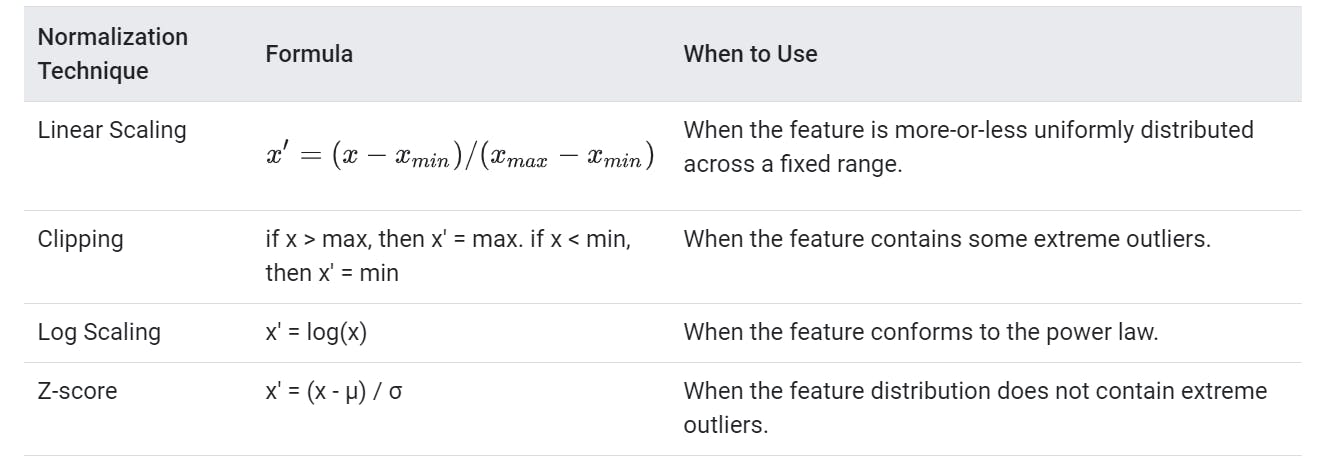
The goal of normalisation is to transform features to be on the same scale in order to stabilise training and for ease of convergence There are four common normalisation techniques:

• scaling to a range
• clipping
• log scaling
• z-score

scaling to a range:
x' = (x - xmin)/(xmax -xmin)
scaling to a range is a good choice when:

1. you know the approximate min and max values of the data with few or no outliers
2. your data is approximately uniformly distributed across that range

A good example for scaling is age. a bad example is income.

Feature Clipping:
if your data contains outliers, feature clipping is appropriate. take for example, you might decide to cap all temperatures above 40 to be exactly 40. Feature clipping caps all feature values above a certain value to a fixed value.
feature clipping can be done before or after normalisations.
you could clip by z-score, i.e +-Nσ e.g. ( limit to +-3σ).

log scaling:
x' = log(x)
log scaling is appropriate if a handful of your values have many points while most other values have few points i.e. a power law distribution.
log scaling improves the performance of linear models

z-score:
x' = (x-μ)/σ
z-score represents the number of standard deviations away from the mean.
you would use z-score to ensure your features have mean=0 and standard deviation=1(similar to transformation by batch)
z-score is useful when there are a few outliers but not so much that you need clipping

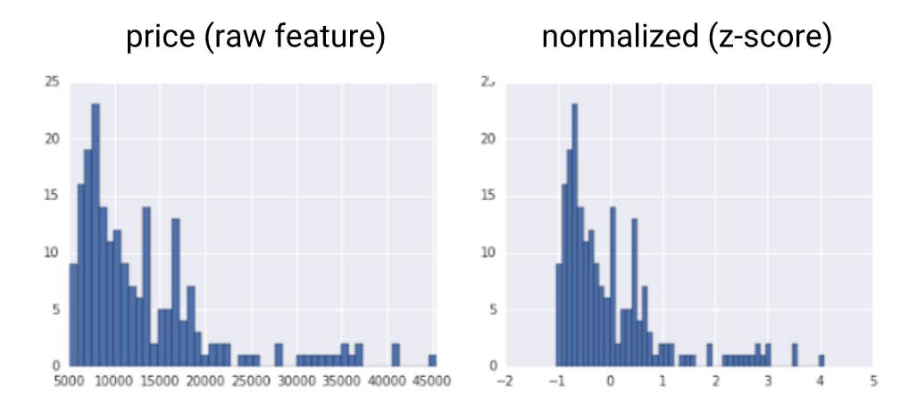
z-score squeezes raw values that have a very large range to a very small range(see image)

how to decide whether to use z-score:

1. if you're not sure wheter the outliers are truly extreme, start with z-score unless you have feature values that you dont want the model to learn.
   finally:
   

Bucketting

is this idea that sometimes the relationship between a feature and a label might not be linear although they are related e.g. the relationship between latitude and housing values. Therefore the feature values are broken down into buckets.
In the case of the latitude v housing values example, we break down latitudes into buckets to learn something different about housing values for each bucket
this means that we will be transforming numeric features into categorical features. this is called bucketting

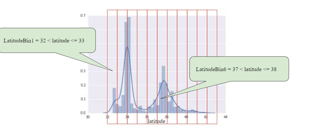
In the example of latitude v housing values(see image), the buckets are evenly spaced.

Quantile Bucketting

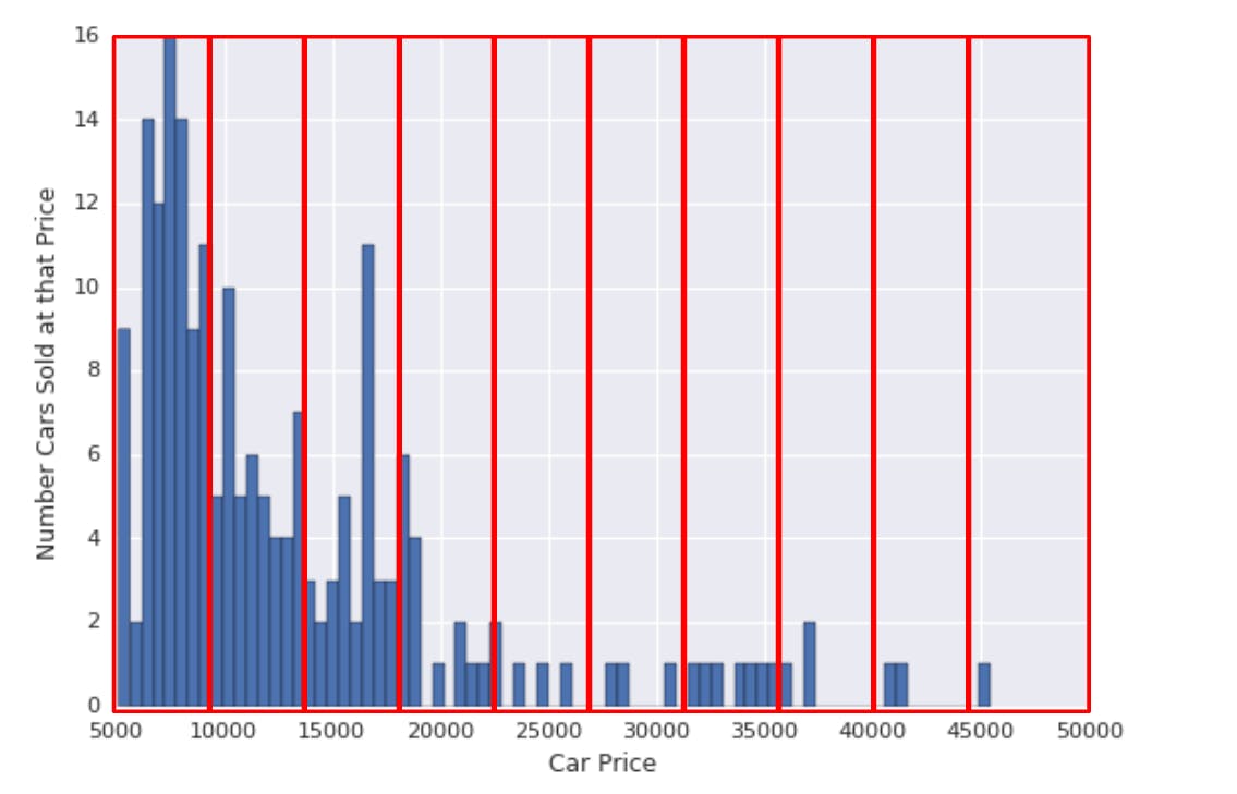
In the above picture, all the buckets are of the same space even though they do not all capture the same amount of data capacity/number of points. This results in waste.

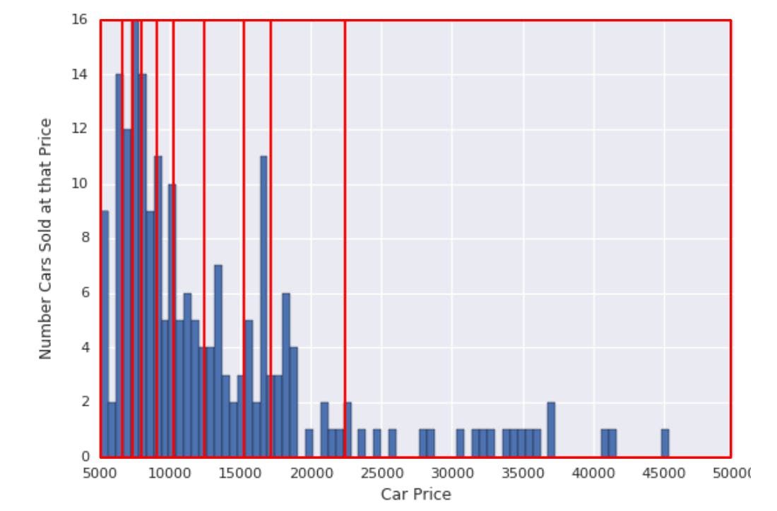
True equality of the buckets comes from ensuring they all capture the same number of points/data capacity. this is the idea behind quantile bucketting

In all, there are two types of buckets:

1. buckets with equally spaced boundaries and
2. quantile buckets in which equality comes from considering the number of points in each bucket

Transforming Categorical Data

Oftentimes, you should represent features that contain integer values as categorical data instead of as numerical data

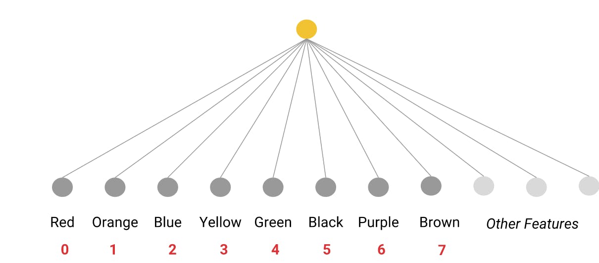
If the number of categories of a data field is small, such as the day of the week or a limited palette of colors, you can make a unique feature for each category

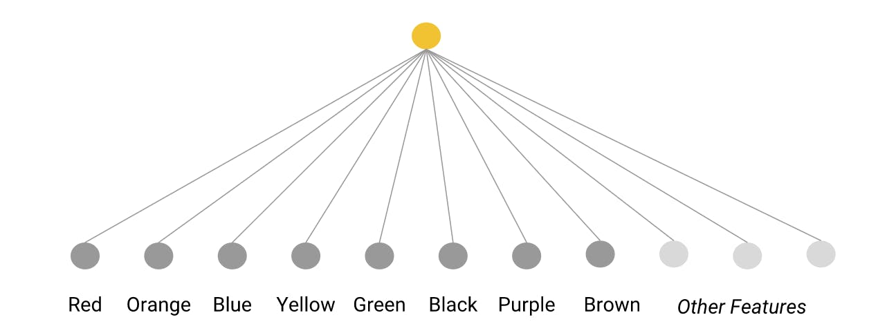
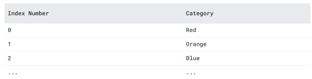
A model can then learn a separate weight for each category and the features can be indexed(mapped to numeric values) thereby creating a vocabulary

one-hot encoding is commonly employed to encode categorical data to transform them into numeric data.
Most implementations in ML will use a sparse representation to keep from storing too many zeros in memory.
OOV out of vocabulary: is used to represent the outliers in categorical data.

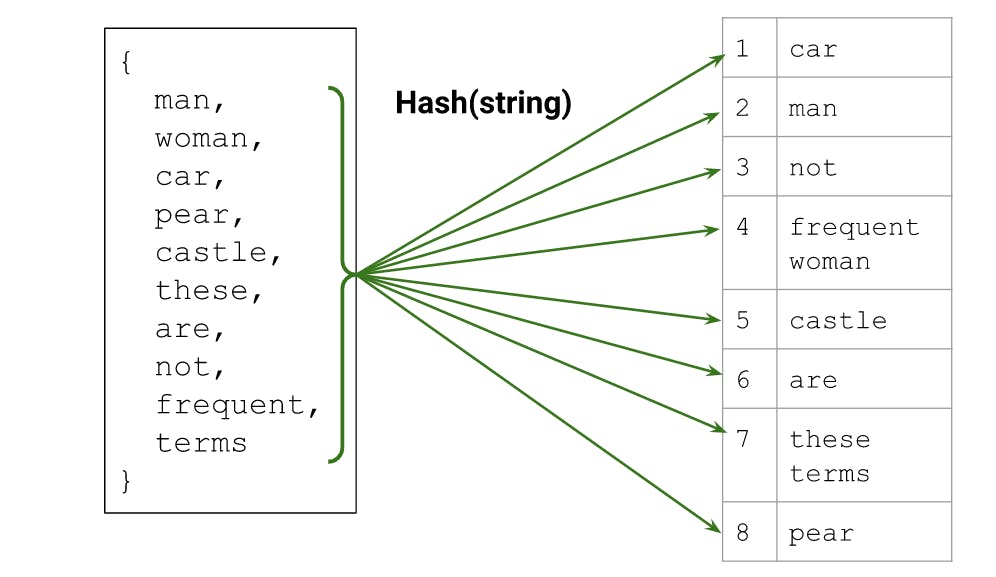
Hashing: can also be used instead of creating a vocabulary. It involves hashing every string into your available index space. It often causes collisions because you are relying on your model to create a representation of the category in the same index that works well for the problem. not having to create a vocab is advantageous especially if the feature distribution changes heavily over time.

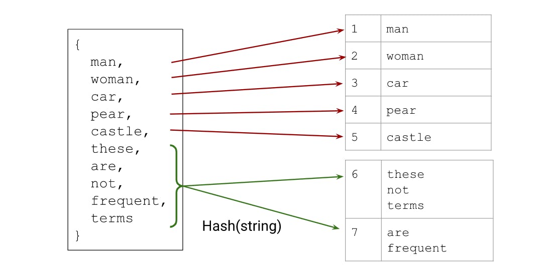
hybrid of hashing and vocab:
we can combine hashing with a vocab.

All the above transformations can be stored on a disk

Embeddings

embeddings are categorical features represented as a continuous value feature. Deep models usually convert the the indices to an embedding.

embeddings cannot be stored on a disk because its trained therefore its part of the model. They are trained with other model weights and functionally are equivalent to a layer of weights

pretrained embeddings are still typically modifiable during training, ergo they are still technically part of the model