I am currently covering all bases in AI/ML before starting my neural networks journey. Part of that is the data manipulation, cleaning and pre-processing I've done for the better part of the last 2 months. Now I am studying the underlying algorithms behind classical ML algorithms. First stop, linreg

classical ml algorithms include those used for supervised, unsupervised and reinforcement learning. supervised learning algorithms include those for regression and classification. The linear regression algorithm deals with numbers. Its aim is to find the relationship between an independent variable(or multiple independent variables) and a dependent variable.

The equation of a line

The four cases of finding the best fit for the linear model

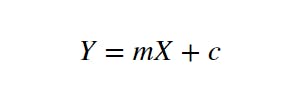
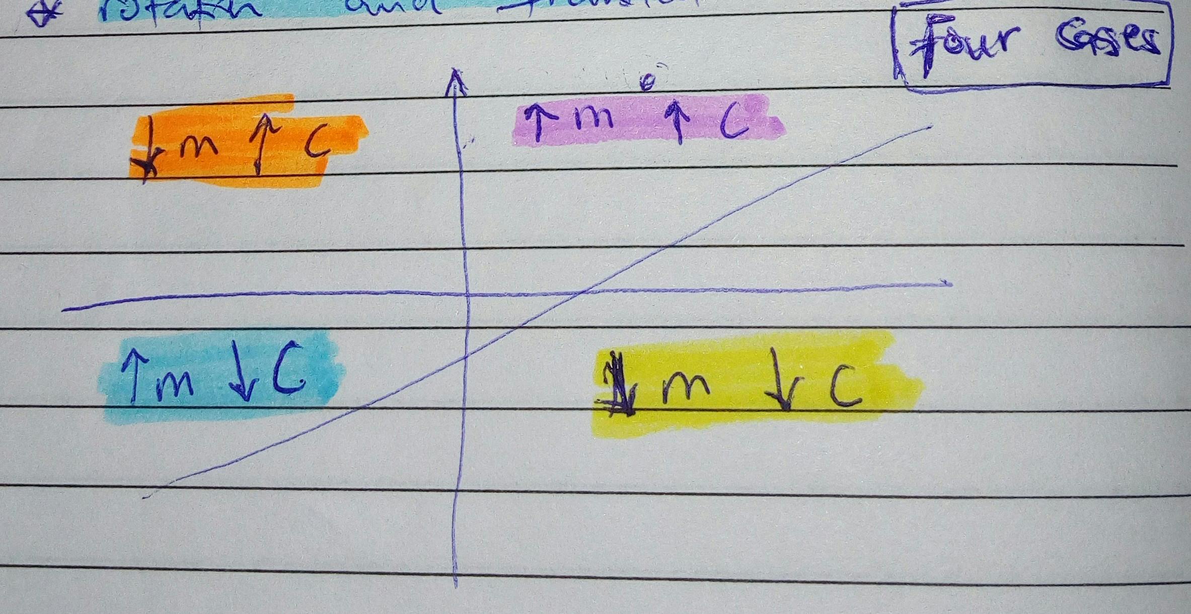
The equation of a line is shown above. The purpose of the linear regression model is to find the best line that represents the data. We do this by repeatedly modifying a random line through rotation and translation.

rotation --> modifying m
translation --> modifying c

The different ways/rules for modifying these two variables depend on the location of the data-point in the x-y coordinate as shown in the diagram above:
The algorithm goes thus:

1. start with a random line
2. pick the epoch(number of iterations)
3. pick the learning rate(a really small number)
4. LOOP(repeat number of epoch times):
   • pick a random point(data-point)
   • if the point is above the line and to the right of the y-axis, rotate counterclockwise and translate up. i.e ↑m↑c
   • if the point is above the line and to the left of the y-axis --> ↓m↑c
   • if the point is below the line and to the right of the y-axis --> ↓m↓c
   • if the point is below the line and to the left of the y-axis --> ↑m↓c
5. enjoy your fitted line❣

def firstlinregmodel(x, y, epoch, lr, x_test):
    """
    lr = learning rate
    epoch = num of batches
    x : array-like, shape = [n_samples, n_features]
        Training samples
    y : array-like, shape = [n_samples, n_target_values]
        Target values
    both x and y are series. x is assumed to be just one series

    ****each datapoint has a vertical and horizontal distance
    """
    # y = mx + c

    # pick a random line
    # which is to say pick random numbers for m and c
    m = 0
    c = 0
    # make the values into data points with vertical and horizontal distance
    data = dict(zip(x, y))

    for _ in range(epoch):
        # to pick a random point
        x_random, y_random = random.choice(list(data.items()))

        # if the point is above the line and to the right of the y axis
        if (m*x_random)+c-y_random > 0 and x_random > 0:
            m += lr
            c += lr
        # if the point is above the line and to the left of the y axis
        elif (m*x_random)+c-y_random > 0 and x_random < 0:
            m -= lr
            c += lr
        # if the point is below the line and to the left of the y axis
        elif (m*x_random)+c-y_random < 0 and x_random < 0:
            m -= lr
            c -= lr
        # if the point is below the line and to the right of the y axis
        elif (m*x_random)+c-y_random < 0 and x_random > 0:
            m += lr
            c -= lr

The code for this algorithm is available here

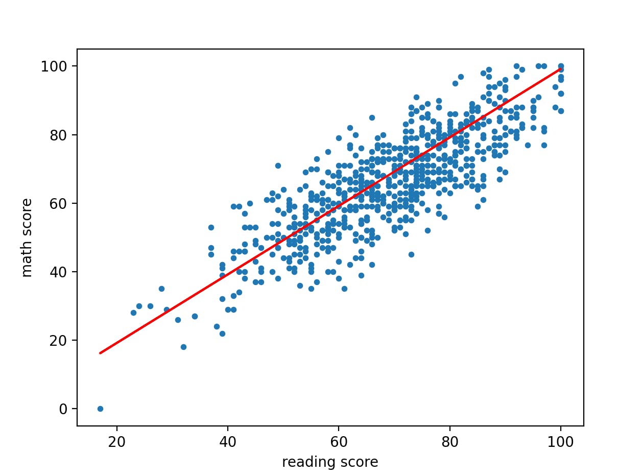
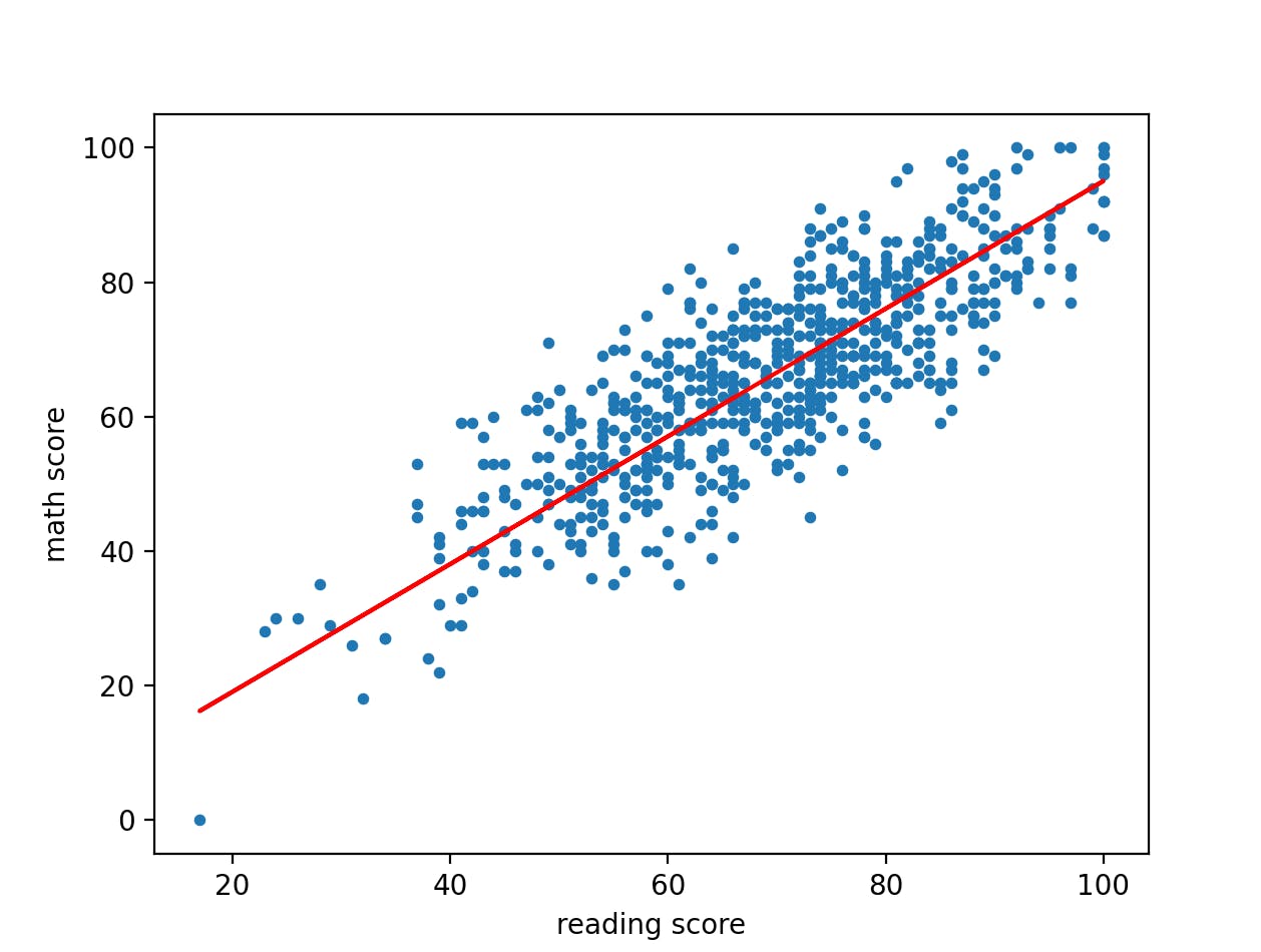
Testing out this algorithm to confirm that it works, we use a student performance data :

data = pd.read_csv('stuperf.csv')
train_data = data[0:700]
test_data = data[700:]
y = train_data['math score']
# y = y.values.reshape((700, 1))
x = train_data['reading score']
# x = x.values.reshape((700, 1))
x_test = test_data['reading score']

print(firstlinregmodel(x, y, 1000, 0.001, x_test))

and we obtain this graph:

Linear Regression Algorithm using Gradient Descent

Gradient descent algorithm is one that is applicable across different parts of ML and even in neural networks. It takes advantage of the difference between the predicted values and the actual values(i.e the residuals/cost) and tries to minimize them as much as possible.
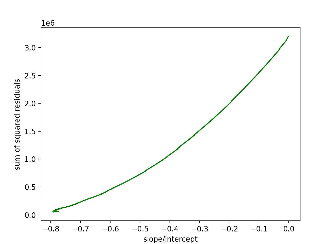
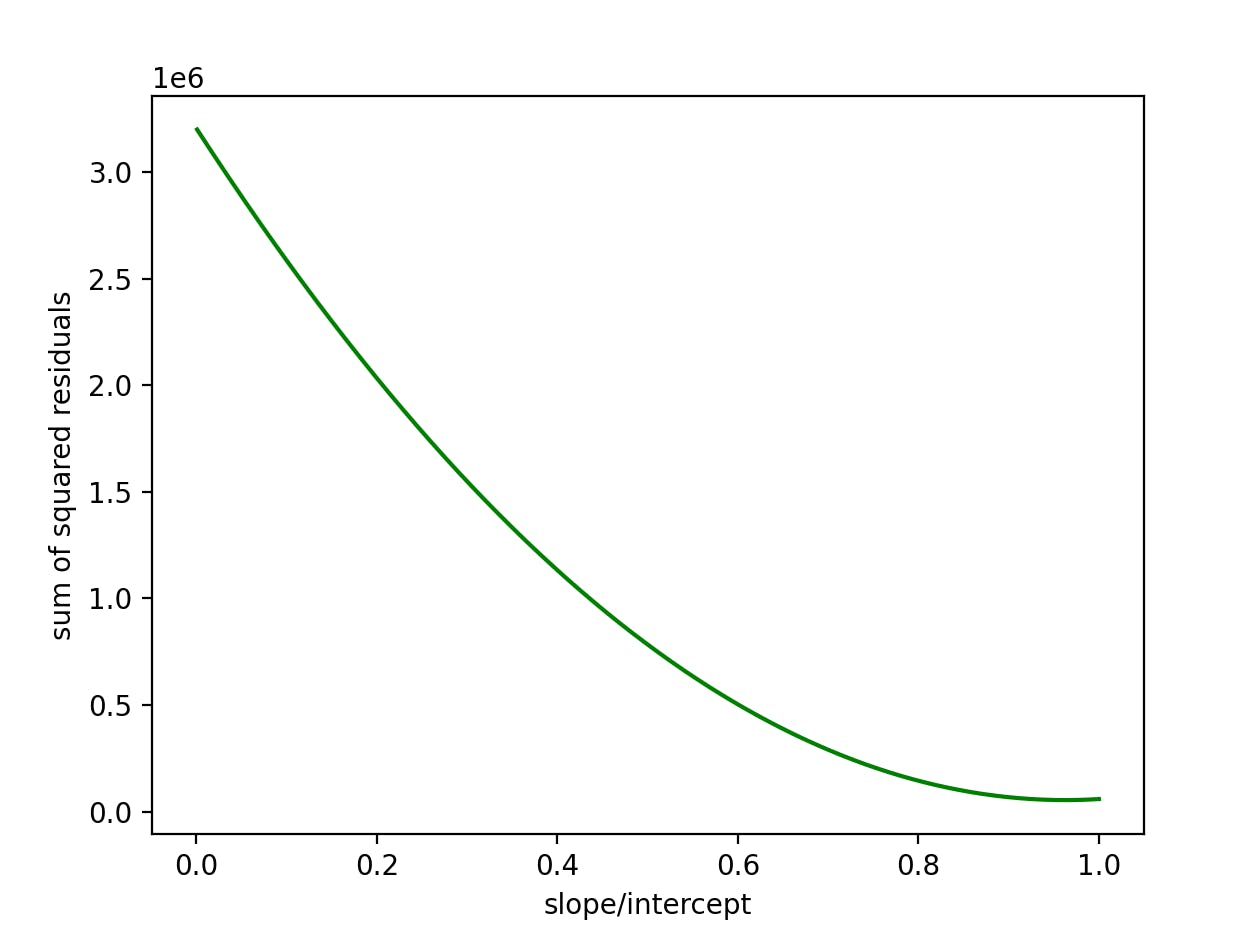
In linear regression, The gradient descent curve is a concave curve representing the cost vs the slope/intercept in a linear regression model.
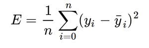
In linear regression, the loss function can be determined using the mean squared error

mean squared error

Least squares
The fastest way to determine the minima of a linear regression algorithm i.e where the error wrt the slope is exactly 0

Gradient descent does the same thing but in a series of iterative steps (the learning rate). The steps are big when far from the minima and small when close to it.

In linear regression, gradient descent is taken wrt both the intercept and the slope i.e we calculate the minima wrt both m and c

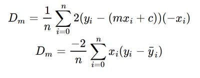
So we find the derivative of the loss function (in this case the mean squared error) wrt both m and c.

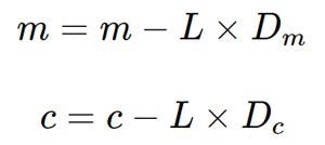
Then we update the values of m and c by essentially taking the steps toward the minima.

So here's the linear regression algorithm using gradient descent:

1. pick initial values for m and c
2. determine the predicted values with the initial values of m and c
3. pick the values for the epoch and learning rate.
4. calculate the partial derivatives wrt m and c using the equations above
5. update the values of m and c using the equation above
6. enjoy your fitted line

The code:

from sklearn.metrics import mean_squared_error, r2_score
from sklearn.linear_model import LinearRegression
import numpy as np
import pandas as pd
import matplotlib.pyplot as plt
import math
import random
from sympy import Symbol, Derivative


def mygradientdescent(X, Y, epoch, L):
    m = 0
    c = 0
    n = float(len(X))  # Number of elements in X
    # Performing Gradient Descent

    for _ in range(epoch):
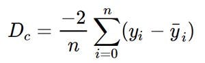
        Y_pred = m*X + c  # The current predicted value of Y
        D_m = (-2/n) * sum(X * (Y - Y_pred))  # Derivative wrt m
        D_c = (-2/n) * sum(Y - Y_pred)  # Derivative wrt c
        m = m - L * D_m  # Update m
        c = c - L * D_c  # Update c
        #print(m, c)
    Y_pred = m*X + c

    plt.scatter(X, Y, s=10)
    plt.plot(x, Y_pred, color='r')  # predicted
    plt.xlabel('reading score')  # x
    plt.ylabel('math score')  # y
    plt.show()
    return


data = pd.read_csv('stuperf.csv')
train_data = data[0:700]
test_data = data[700:]
y = train_data['math score']
# y = y.values.reshape((700, 1))
x = train_data['reading score']
# x = x.values.reshape((700, 1))
x_test = test_data['reading score']

mygradientdescent(x, y, 1000, 0.00001)

we obtain this graph:

The code for this algorithm is also available here

Gradient descent is useful when it is not possible to solve for where the derivative of the curve is 0 like in least squares. so I imagine in cases where there are many minima and its difficult to determine the best one -- neural networks

NOTES for me 🧾:

1. gradient descent deals with the negative derivative of the tangent to a point on the curve.
2. step size = slope of the current point * learning rate
3. new intercept = old intercept - step size
4. gradient descent depends on the loss function
5. the gradient descent curve is a graph of the sum of squared loss/residuals vs the slope/intercept(or the determining factor(s)/variables for the fit of your model)

for our linear regression model above, the gradient descent curves wrt both slope and intercept are:

gradient descent curve wrt intercept

gradient descent curve wrt slope

References:

1. luis serrano's youtube
2. statquest with josh stammer